3. Detect Holo-like Conformations from an Apo Trajectory#
FragBEST-Myo is a specific version of FragBEST (Fragment-Based protein Ensemble semantic Segmentation Tool). The model is trained with omecamtiv mecarbil (OM)-bound PPS/PR-state cardiac myosin trajectories. The model enables to predict the protein’s surfacial region potential binding with the chemical fragments of OM. This information is further utilized for detecting holo-like conformations by converting it into holo descriptors and selecting the top-ranked conformations.
Here, we demonstrate how to detect and select holo-like conformations from an apo trajectory.
In this tutorial, you will learn:
How to load and analyze the apo trajectory with our class objects
TrajectoryHandler,HoloDescriptor, andHoloDescriptorAnalyser.How to use parallel processing class object
TrajHandlerPreprocessandTrajHandlerPredictionto work on the full trajectory.How to identify the holo-like conformation from an apo trajectory.
Set up the environment and path#
# only for once to append the root of the project
import os
import sys
import warnings


def find_project_root(marker=".git"):
    current_path = os.getcwd()
    while current_path != os.path.dirname(current_path):  # Stop at the filesystem root
        if marker in os.listdir(current_path):
            return current_path
        current_path = os.path.dirname(current_path)
    return None  # Return None if the marker is not found


project_root = find_project_root()
print(project_root)
# should be at the root of the project
# e.g., /.../.../.../FragBEST-Myo

# Add project_root to the Python path
sys.path.append(project_root)

# ignore warnings
warnings.filterwarnings("ignore")
/home/yuyang/Project_local/FragBEST-Myo
# import the necessary packages
from IPython.display import HTML, Image, display
from natsort import natsorted

from utils.datasets.general import add_prediction_to_ply, preprocess_workflow
from utils.datasets.traj_handler import TrajectoryHandler
from utils.parallel.framework import (
    TrajHandlerPrediction,
    TrajHandlerPreprocess,
    TrajHandlerVisualization,
)
from utils.ppseg.holo_descriptor.holo_descriptor import HoloDescriptorAnalyser
from utils.pymol_scripts.vis_pdb_ply import generate_pse, merge_pse


def display_df_html(df):
    """
    Display a pandas DataFrame as HTML in Jupyter Notebook.
    """
    for each in df:
        # check if the column is a list
        if isinstance(df[each].iloc[0], list):
            # convert the list to a string
            # (use two decimal places and format it as a string)
            df[each] = df[each].apply(
                lambda x: "[" + ",".join([f"{i:.2f}" for i in x]) + "]"
            )
    display(HTML('<div style="overflow-x: auto">' + df.to_html() + "</div>"))
Attention
It is recommended to use absolute path to indicate the file. Especially in generating the surface files.
Important
For your topology file, the residues should be in the standard residue name. For instannce, histidine should be HIS rather than HID, HIE, or HIP. Otherwise, MSMS will not recognized those histidines.
Load the inputs and create a output directory#
In this tutorial, we used two input files for the apo trajectory. These data can be downloaded from our Zenodo.
Apo_SMD_T300_p_fit.pdb: the topology file.Apo_SMD_200ns_skip10ns.xtc: the trajectory file. It is a steered-MD trajecotry of cardiac myosin from post-rigor (PR) to pre-power-stroke (PPS)-like state. The simulation time is 200 ns and this trajectory is saved with 10 ns interval. In total, there are around 20 frames.
We also used two input files for the reference state of the cardiac myosin, which can be found in FragBEST-Myo/dataset/ref folder.
PPS_OMB_min_cg_pl.pdb: the reference structure to align the apo trajectory on it. Note that the reference structure is pre-power-stroke (PPS) state cardiac myosin with omecamtiv mecarbil.pocket_aux.txt: the pocket auxiliary file generated from the reference structure.
# -------------- Start of user-defined variables --------------
top_path = f"{project_root}/dataset/examples/Apo_SMD_aligned_PPS_converted.pdb"
traj_path = f"{project_root}/dataset/examples/Apo_SMD_200ns_skip10ns.xtc"

ref_path = f"{project_root}/dataset/ref/PPS_OMB_min_cg_pl.pdb"
ref_aux_path = f"{project_root}/dataset/ref/pocket_aux.txt"

output_dir = f"{project_root}/dataset/examples/outputs_holo_like"
# -------------- End of user-defined variables ----------------

# Create output directory
os.makedirs(output_dir, exist_ok=True)
# Download the files from zenodo
!wget -O {top_path} https://zenodo.org/record/19822671/files/Apo_SMD_aligned_PPS_converted.pdb
!wget -O {traj_path} https://zenodo.org/record/19822671/files/Apo_SMD_200ns_skip10ns.xtc
Now, let’s load the reference structure and the apo trajectory with TrajectoryHandler. We also read the pocket auxiliary file (which is provided in advance) to traj_handler.
Then, the apo trajectory is aligned to the reference structure by traj_handler.aligna_traj_to_procket with reference=ref.universe. This function uses the pocket residue IDs to select the atom group and align the apo trajectory to the reference structure. By default, after alignment, the pocket center is also updated based on the pocket residues. However, in this tutorial, the pocket center has already been calculated based on the reference. Thus, we set update_pocket_center=False.
# Load reference structure
ref = TrajectoryHandler(ref_path, ligand_name="2OW", warning_check=False)

# Load trajectory
traj_handler = TrajectoryHandler(
    top_path, traj_path, ligand_name=None, warning_check=False
)

# Load the pocket aux file
traj_handler.read_pocket_aux_file(ref_aux_path)

# Align the trajectory to the reference structure
traj_handler.align_traj_to_pocket(reference=ref.universe, update_pocket_center=False)

# Print the pocket residues and the pocket center
print(f"pocket residues: {traj_handler.residues_at_pocket_str}")
print(f"pocket center: {traj_handler.pocket_center}")
pocket residues: 120 146 147 160 163 164 167 168 170 492 497 666 667 710 711 712 713 721 722 765 770 771 774
pocket center: [48.24788948519146, 107.53731136226175, 63.72042723995956]
Note:
The provided pocket auxiliary file was prepared from the reference structure using the following code snippet:
# Obtain the pocket center from the reference structure
ref.get_pocket_center()  # Get the pocket center coordinates

# Write the pocket auxiliary file to the specified path
ref.write_pocket_aux_file(ref_aux_path)  # Save the pocket auxiliary file
If you are working with skeletal myosin or another isoform, the provided reference structure may not be suitable for your analysis. To deal with those cases, check the advanced usage note here to align the trajectory to the first frame.
Now, let’s check the region of interest in nglview.
# import nglview package
# (uncomment below code to visualize the structure)

# import nglview as nv

# view = nv.show_mdanalysis(traj_handler.universe)  # visualize the structure
# view.shape.add(
#     "sphere",
#     list(traj_handler.pocket_center),
#     [0.5, 0.5, 0.5],
#     traj_handler.radius_of_interest,
#     f"region of interest with {traj_handler.radius_of_interest} angstrom radius",
# )  # the interest of region with 16.0 angstrom radius and the pocket center
# view
Preprocess Data in Parallel#
To preprocess data in parallel, follow the steps below to generate PDB, PLY, and H5 files for each conformation.
1. Initialize TrajHandlerPreprocess#
Use TrajHandlerPreprocess to manage the parallel jobs. When initializing, set the max_workers parameter to specify the number of threads you want to use. You can determine the optimal number of threads for your system by using tools like htop in your terminal.
Hint
If you encounter a memory usage issue, consider reducing your max_workers. Setting it to 4 or 8 may resolve the problem on your machine.
2. Prepare Inputs#
Call TrajHandlerPreprocess.prepare() to prepare the input data.
The trajectory will be split into multiple PDB, PLY, and H5 files. For example:
The PDB file for frame
0will be saved as/[root_path]/[filename]_0.pdb.The corresponding PLY and H5 files will be saved in the same directory with the same base filename but different extensions (
.plyand.h5).
Important
By using the method demonstrated here, you need to manually define the following parameters:
root_path: The directory where the processed files will be saved.filename: The base name for each conformation file.
If you would like to use the configuration-based method, root_path and filename are optional. We will demonstrate how to use a configuration-based method to run the pipeline in advanced usage.
3. Run the Workflow#
For most use cases, the preprocess_workflow function is the main function to execute the entire preprocessing workflow. This includes:
Generating PDB, PLY, and H5 files.
Creating an index file to record the processed conformations.
To configure the workflow, use the TrajHandlerPreprocess.set_function() method. This allows you to define the function and pass common arguments.
By following these steps, you can efficiently preprocess your trajectory data in parallel, ensuring all necessary files are generated and properly organized.
# ----------- Start of user-defined variables ------------
logger_path = f"{output_dir}/core-dataprep-info.log"
max_workers = 16
filename_p = "Apo_SMD_protein"  # filename base for each conformation
# ----------- End of user-defined variables --------------

# Prepare to run the dataset preprocessing
p_jobs = TrajHandlerPreprocess(max_workers=max_workers, logger_path=logger_path)
p_jobs.prepare(
    traj_handler,
    root_path=output_dir,
    filename=filename_p,
)

# set the function
p_jobs.set_function(preprocess_workflow)

# run the preprocessing workflow
p_jobs.run()  # this takes around 3.5 minutes
2026-05-06 12:05:05,917 core-dataprep INFO: Preprocess: 8 done
2026-05-06 12:05:07,189 core-dataprep INFO: Preprocess: 11 done
2026-05-06 12:05:10,708 core-dataprep INFO: Preprocess: 10 done
2026-05-06 12:05:25,175 core-dataprep INFO: Preprocess: 7 done
2026-05-06 12:05:29,385 core-dataprep INFO: Preprocess: 12 done
2026-05-06 12:05:30,713 core-dataprep INFO: Preprocess: 9 done
2026-05-06 12:05:31,981 core-dataprep INFO: Preprocess: 13 done
2026-05-06 12:05:33,264 core-dataprep INFO: Preprocess: 1 done
2026-05-06 12:05:34,393 core-dataprep INFO: Preprocess: 4 done
2026-05-06 12:05:35,236 core-dataprep INFO: Preprocess: 6 done
2026-05-06 12:05:38,657 core-dataprep INFO: Preprocess: 0 done
2026-05-06 12:05:39,572 core-dataprep INFO: Preprocess: 3 done
2026-05-06 12:05:41,691 core-dataprep INFO: Preprocess: 14 done
2026-05-06 12:05:45,030 core-dataprep INFO: Preprocess: 15 done
2026-05-06 12:05:46,655 core-dataprep INFO: Preprocess: 2 done
2026-05-06 12:05:47,672 core-dataprep INFO: Preprocess: 5 done
2026-05-06 12:06:30,020 core-dataprep INFO: Preprocess: 16 done
2026-05-06 12:06:45,858 core-dataprep INFO: Preprocess: 17 done
2026-05-06 12:06:50,118 core-dataprep INFO: Preprocess: 18 done
2026-05-06 12:07:00,906 core-dataprep INFO: Preprocess: 19 done
2026-05-06 12:07:01,925 core-dataprep INFO: Preprocess: 20 done
Now, you have completed the preprocess of the data.
Some optional parameters can be adjusted, check here for more details.
Make Predictions in Parallel#
Similar to data preprocessing, predictions can also be performed using parallel processors for increased efficiency.
Here, we use TrajHandlerPrediction instead of TrajHandlerPreprocess. The TrajHandlerPrediction class inherits most attributes from TrajHandlerPreprocess but includes minor modifications. Additionally, we utilize the add_prediction_to_ply function to make predictions.
Preparation Steps
Similar to the preprocessing step, you need to define the following:
root_path: The root directory containing the trajectory files.filename: The name of the file(s) to process.
When running the function, you’ll also need to include the following parameters:
model_path: Path to the pretrained model checkpoint used for making predictions.
# ----------- Start of user-defined variables ------------
logger_path = f"{output_dir}/core-predict-info.log"
max_workers = 16
filename_p = "Apo_SMD_protein"  # filename base for each conformation
model_path = f"{project_root}/utils/ppseg/myo/Kfold3_best_model_187_miou=0.7492.pt"
# ----------- End of user-defined variables --------------

# Prepare to run the dataset preprocessing
p_jobs = TrajHandlerPrediction(max_workers=max_workers, logger_path=logger_path)
p_jobs.prepare(traj_handler, root_path=output_dir, filename=filename_p)

# set up the function
p_jobs.set_function(
    func=add_prediction_to_ply,
    model_path=model_path,
)

# run the preprocessing workflow
p_jobs.run()  # this takes around 1 minute"
2026-05-06 12:07:48,028 core-predict INFO: Prediction: 8 done
2026-05-06 12:07:49,180 core-predict INFO: Prediction: 6 done
2026-05-06 12:07:49,248 core-predict INFO: Prediction: 0 done
2026-05-06 12:07:49,343 core-predict INFO: Prediction: 9 done
2026-05-06 12:07:50,132 core-predict INFO: Prediction: 11 done
2026-05-06 12:07:50,444 core-predict INFO: Prediction: 1 done
2026-05-06 12:07:50,999 core-predict INFO: Prediction: 3 done
2026-05-06 12:07:51,247 core-predict INFO: Prediction: 2 done
2026-05-06 12:07:51,402 core-predict INFO: Prediction: 10 done
2026-05-06 12:07:51,554 core-predict INFO: Prediction: 5 done
2026-05-06 12:07:52,490 core-predict INFO: Prediction: 7 done
2026-05-06 12:07:53,489 core-predict INFO: Prediction: 13 done
2026-05-06 12:07:55,543 core-predict INFO: Prediction: 12 done
2026-05-06 12:07:56,549 core-predict INFO: Prediction: 14 done
2026-05-06 12:07:58,717 core-predict INFO: Prediction: 15 done
2026-05-06 12:07:59,647 core-predict INFO: Prediction: 4 done
2026-05-06 12:08:01,992 core-predict INFO: Prediction: 16 done
2026-05-06 12:08:03,163 core-predict INFO: Prediction: 17 done
2026-05-06 12:08:04,564 core-predict INFO: Prediction: 20 done
2026-05-06 12:08:04,656 core-predict INFO: Prediction: 19 done
2026-05-06 12:08:04,863 core-predict INFO: Prediction: 18 done
In default, cpu is used for the prediction. If you wish to use cuda for prediction, check the optional parameters for prediction here for more details.
Important
We expect your GPU is compatible with CUDA 12. If FragBEST-Myo doesn’t work with GPU, please use cpu instead.
Analyze the Results#
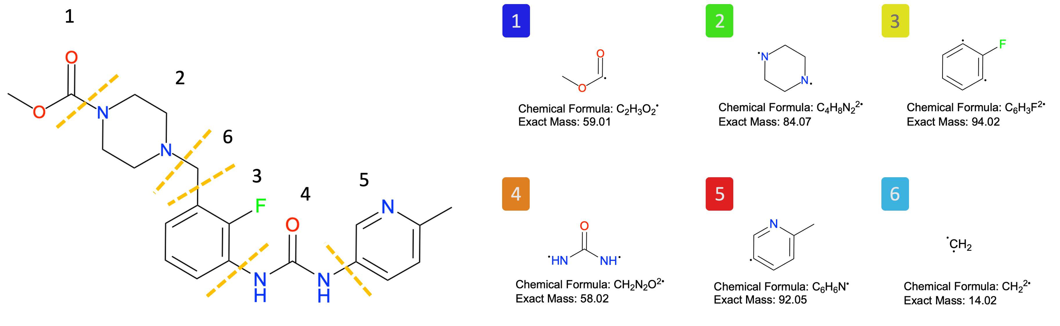
To analyze the results, we use the HoloDescriptorAnalyser. Since FragBEST-Myo was trained with predefined fragments (see the figure), the corresponding fragment information was prepared beforehand. This information is also available in the example file located at FragBEST-Myo/utils/ppseg/myo/ligand_fragments_example.json (loaded by default).
# visualization of fragments
Image(filename=f"{project_root}/imgs/OM_fragment.png")
The source_path parameter should point to the directory where you have saved the required files (JSON). After setting up the paths, follow these steps:
List the files: Use
self.list_files()to generate a list of relevant files.Read the files: Load the files and enable HoloSpace calculation by using
self.read(holospace_calc=True).Perform z-score normalization: Normalize the data with
self.calculate_zscore()using the following four recommended descriptors:num_of_classes(D1)nonbck_ratio(D2)nonbck_class_pt_ratio(D3)holospace_frag_score(D4)
Set the rank: Rank the results using
self.set_rank()with equal weights (default setting) and prioritize the conformations without warnings by settingfilter_warning=True.Select top N results: Select top N conformations using
self.set_n().
For further details about HoloDescriptor, refer to the Tutorial 2.
# source_path having the holo-descriptor json files
hd_analyser = HoloDescriptorAnalyser(source_path=output_dir)

# list the files
hd_analyser.list_files()

# read the multiple holo descriptor files
hd_analyser.read(holospace_calc=True)

# calculate the z-score of the selected holo descriptors (without preset)
hd_analyser.calculate_zscore("num_of_classes")
hd_analyser.calculate_zscore("nonbck_ratio")
hd_analyser.calculate_zscore("nonbck_class_pt_ratio")
hd_analyser.calculate_zscore("holospace_frag_score")

# set the rank
hd_analyser.set_rank(filter_warning=True)
Found 21 files
In total, 21 files are expected to be found (21 different conformations). With the filter_warning, the conformations that produce warnings will be assigned a lower rank.
# display top 5 conformations
display_df_html(hd_analyser.top_n(5))
| class_predprobs | overall_predprobs | class_pt_ratio | nonbck_ratio | nonbck_class_pt_ratio | num_of_classes | num_interest_points | holospace_volume | holospace_frag_volumes | filename | warnings | holospace_frag_score | num_of_classes_zscore | nonbck_ratio_zscore | nonbck_class_pt_ratio_zscore | holospace_frag_score_zscore | overall_score | rank | |
|---|---|---|---|---|---|---|---|---|---|---|---|---|---|---|---|---|---|---|
| 20 | [1.00,1.00,1.00,0.97,0.98,0.97,1.00] | 0.994042 | [0.79,0.05,0.03,0.03,0.04,0.03,0.02] | 0.208368 | 0.034728 | 7 | 1219 | 1617.916439 | [200.39,306.48,351.01,285.53,401.45,82.51] | Apo_SMD_protein_20.json | 1.0 | 1.208081 | 1.292830 | 0.732379 | 1.734074 | 1.241841 | 1 | |
| 19 | [1.00,0.95,1.00,0.99,0.97,0.98,1.00] | 0.992693 | [0.79,0.02,0.03,0.04,0.04,0.08,0.01] | 0.206926 | 0.034488 | 7 | 1155 | 1240.567267 | [29.06,59.12,371.24,304.42,394.51,19.11] | Apo_SMD_protein_19.json | 0.829463 | 1.208081 | 1.261689 | 0.702718 | 0.813435 | 0.996481 | 2 | |
| 1 | [0.99,0.97,0.00,0.92,0.98,0.94,0.95] | 0.981299 | [0.81,0.03,0.00,0.06,0.05,0.04,0.02] | 0.190941 | 0.038188 | 6 | 1126 | 1398.913503 | [95.93,0.00,291.81,473.78,392.51,59.29] | Apo_SMD_protein_1.json | 0.833333 | -0.201347 | 0.916264 | 1.159702 | 0.834329 | 0.677237 | 3 | |
| 15 | [0.99,0.96,0.93,0.91,0.95,0.90,1.00] | 0.980827 | [0.83,0.02,0.01,0.03,0.05,0.04,0.01] | 0.167438 | 0.027906 | 7 | 1081 | 2036.372888 | [75.76,12.19,678.45,209.80,292.47,26.84] | Apo_SMD_protein_15.json | 0.856336 | 1.208081 | 0.408364 | -0.110035 | 0.958507 | 0.616229 | 4 | |
| 17 | [0.99,0.97,0.93,0.93,0.95,0.94,0.94] | 0.984131 | [0.84,0.02,0.02,0.02,0.04,0.05,0.01] | 0.163951 | 0.027325 | 7 | 982 | 1208.181939 | [43.31,63.92,277.18,252.99,569.48,13.96] | Apo_SMD_protein_17.json | 0.846251 | 1.208081 | 0.333024 | -0.181792 | 0.904064 | 0.565844 | 5 |
From the results, 10 conformations were identified without warnings. By rank, the top 5 frames are 20, 19, 1, 15, and 17 which represent time points 200 ns, 190 ns, 10 ns, 150 ns, and 170 ns, respectively.
Key Insight:
Higher-ranked conformations (e.g., frame
20>19>1>15>17) have a higher probability of being holo-like conformations.These conformations are considered valuable protein ensembles and can be selected for further drug design studies.
By prioritizing these frames, you can focus on structures most likely to contribute to effective drug discovery.
Visualization#
For visualizing individual structures, you can use PyMOL to open the PLY file with our plugin: FragBEST PyMOL Plugin. This plugin enables detailed visualization of features, labels, and predicted points on the protein surface.
Alternatively, refer to Tutorial 1 - Visualization with PyMOL to learn how to generate .pse visualization files with the code.
Batch Visualization with Parallel Processing
You can also use a parallel processor to generate .pse files for multiple structures simultaneously. After generating individual visualization files, you can merge all the .pse files into a single .pse file for comprehensive visualization.
This approach simplifies the visualization process for large protein ensembles and provides an efficient way to analyze multiple structures in one view.
Step 1: Set Up a Parallel Processor to Generate Multiple Files#
Similar to preprocessing and prediction, you need to configure the following: logger, max_workers, and filename_p (the base name for the protein files). The executable PyMOL is already installed as part of the environment setup.
# ----------- Start of user-defined variables ------------
logger_path = f"{output_dir}/core-vis-info.log"
max_workers = 24
filename_p = "Apo_SMD_protein"  # filename base for each conformation
# ----------- End of user-defined variables --------------

# Set up the pymol path
pymol_path = !pixi run -e pymol which pymol
pymol_path = pymol_path[0]

# Prepare to run the dataset preprocessing
p_jobs = TrajHandlerVisualization(max_workers=max_workers, logger_path=logger_path)
p_jobs.prepare(
    traj_handler,
    root_path=output_dir,
    filename=filename_p,
)

# set the function
p_jobs.set_function(generate_pse, pymol_path=pymol_path)

# run the preprocessing workflow
p_jobs.run()  # this takes around 3 minutes
interest_pt: 1
ignore_surface: 0
pb_vert_Apo_SMD_protein_16.ply pb_surf_Apo_SMD_protein_16.ply hphob_vert_Apo_SMD_protein_16.ply hphob_surf_Apo_SMD_protein_16.ply hbond_vert_Apo_SMD_protein_16.ply hbond_surf_Apo_SMD_protein_16.ply pred_vert_Apo_SMD_protein_16.ply pred_surf_Apo_SMD_protein_16.ply mesh_Apo_SMD_protein_16.ply
2026-05-06 12:16:00,868 core-vis INFO: Generated PyMOL session file: Apo_SMD_protein_16.pse
interest_pt: 1
ignore_surface: 0
2026-05-06 12:16:04,403 core-vis INFO: Generated PyMOL session file: Apo_SMD_protein_8.pse
pb_vert_Apo_SMD_protein_8.ply pb_surf_Apo_SMD_protein_8.ply hphob_vert_Apo_SMD_protein_8.ply hphob_surf_Apo_SMD_protein_8.ply hbond_vert_Apo_SMD_protein_8.ply hbond_surf_Apo_SMD_protein_8.ply pred_vert_Apo_SMD_protein_8.ply pred_surf_Apo_SMD_protein_8.ply mesh_Apo_SMD_protein_8.ply
interest_pt: 1
ignore_surface: 0
2026-05-06 12:16:07,467 core-vis INFO: Generated PyMOL session file: Apo_SMD_protein_17.pse
pb_vert_Apo_SMD_protein_17.ply pb_surf_Apo_SMD_protein_17.ply hphob_vert_Apo_SMD_protein_17.ply hphob_surf_Apo_SMD_protein_17.ply hbond_vert_Apo_SMD_protein_17.ply hbond_surf_Apo_SMD_protein_17.ply pred_vert_Apo_SMD_protein_17.ply pred_surf_Apo_SMD_protein_17.ply mesh_Apo_SMD_protein_17.ply
interest_pt: 1
ignore_surface: 0
2026-05-06 12:16:08,213 core-vis INFO: Generated PyMOL session file: Apo_SMD_protein_14.pse
pb_vert_Apo_SMD_protein_14.ply pb_surf_Apo_SMD_protein_14.ply hphob_vert_Apo_SMD_protein_14.ply hphob_surf_Apo_SMD_protein_14.ply hbond_vert_Apo_SMD_protein_14.ply hbond_surf_Apo_SMD_protein_14.ply pred_vert_Apo_SMD_protein_14.ply pred_surf_Apo_SMD_protein_14.ply mesh_Apo_SMD_protein_14.ply
interest_pt: 1
ignore_surface: 0
2026-05-06 12:16:08,899 core-vis INFO: Generated PyMOL session file: Apo_SMD_protein_0.pse
pb_vert_Apo_SMD_protein_0.ply pb_surf_Apo_SMD_protein_0.ply hphob_vert_Apo_SMD_protein_0.ply hphob_surf_Apo_SMD_protein_0.ply hbond_vert_Apo_SMD_protein_0.ply hbond_surf_Apo_SMD_protein_0.ply pred_vert_Apo_SMD_protein_0.ply pred_surf_Apo_SMD_protein_0.ply mesh_Apo_SMD_protein_0.ply
interest_pt: 1
ignore_surface: 0
interest_pt: 1
ignore_surface: 0
pb_vert_Apo_SMD_protein_15.ply pb_surf_Apo_SMD_protein_15.ply hphob_vert_Apo_SMD_protein_15.ply hphob_surf_Apo_SMD_protein_15.ply hbond_vert_Apo_SMD_protein_15.ply hbond_surf_Apo_SMD_protein_15.ply pred_vert_Apo_SMD_protein_15.ply pred_surf_Apo_SMD_protein_15.ply mesh_Apo_SMD_protein_15.ply
2026-05-06 12:16:12,598 core-vis INFO: Generated PyMOL session file: Apo_SMD_protein_15.pse
2026-05-06 12:16:13,035 core-vis INFO: Generated PyMOL session file: Apo_SMD_protein_7.pse
pb_vert_Apo_SMD_protein_7.ply pb_surf_Apo_SMD_protein_7.ply hphob_vert_Apo_SMD_protein_7.ply hphob_surf_Apo_SMD_protein_7.ply hbond_vert_Apo_SMD_protein_7.ply hbond_surf_Apo_SMD_protein_7.ply pred_vert_Apo_SMD_protein_7.ply pred_surf_Apo_SMD_protein_7.ply mesh_Apo_SMD_protein_7.ply
interest_pt: 1
ignore_surface: 0
2026-05-06 12:16:13,914 core-vis INFO: Generated PyMOL session file: Apo_SMD_protein_4.pse
pb_vert_Apo_SMD_protein_4.ply pb_surf_Apo_SMD_protein_4.ply hphob_vert_Apo_SMD_protein_4.ply hphob_surf_Apo_SMD_protein_4.ply hbond_vert_Apo_SMD_protein_4.ply hbond_surf_Apo_SMD_protein_4.ply pred_vert_Apo_SMD_protein_4.ply pred_surf_Apo_SMD_protein_4.ply mesh_Apo_SMD_protein_4.ply
interest_pt: 1
ignore_surface: 0
interest_pt: 1
ignore_surface: 0
2026-05-06 12:16:15,281 core-vis INFO: Generated PyMOL session file: Apo_SMD_protein_3.pse
2026-05-06 12:16:15,328 core-vis INFO: Generated PyMOL session file: Apo_SMD_protein_2.pse
pb_vert_Apo_SMD_protein_3.ply pb_surf_Apo_SMD_protein_3.ply hphob_vert_Apo_SMD_protein_3.ply hphob_surf_Apo_SMD_protein_3.ply hbond_vert_Apo_SMD_protein_3.ply hbond_surf_Apo_SMD_protein_3.ply pred_vert_Apo_SMD_protein_3.ply pred_surf_Apo_SMD_protein_3.ply mesh_Apo_SMD_protein_3.ply
pb_vert_Apo_SMD_protein_2.ply pb_surf_Apo_SMD_protein_2.ply hphob_vert_Apo_SMD_protein_2.ply hphob_surf_Apo_SMD_protein_2.ply hbond_vert_Apo_SMD_protein_2.ply hbond_surf_Apo_SMD_protein_2.ply pred_vert_Apo_SMD_protein_2.ply pred_surf_Apo_SMD_protein_2.ply mesh_Apo_SMD_protein_2.ply
interest_pt: 1
ignore_surface: 0
interest_pt: 1
ignore_surface: 0
interest_pt: 1
ignore_surface: 0
2026-05-06 12:16:16,215 core-vis INFO: Generated PyMOL session file: Apo_SMD_protein_9.pse
pb_vert_Apo_SMD_protein_9.ply pb_surf_Apo_SMD_protein_9.ply hphob_vert_Apo_SMD_protein_9.ply hphob_surf_Apo_SMD_protein_9.ply hbond_vert_Apo_SMD_protein_9.ply hbond_surf_Apo_SMD_protein_9.ply pred_vert_Apo_SMD_protein_9.ply pred_surf_Apo_SMD_protein_9.ply mesh_Apo_SMD_protein_9.ply
pb_vert_Apo_SMD_protein_19.ply pb_surf_Apo_SMD_protein_19.ply hphob_vert_Apo_SMD_protein_19.ply hphob_surf_Apo_SMD_protein_19.ply hbond_vert_Apo_SMD_protein_19.ply hbond_surf_Apo_SMD_protein_19.ply pred_vert_Apo_SMD_protein_19.ply pred_surf_Apo_SMD_protein_19.ply mesh_Apo_SMD_protein_19.ply
pb_vert_Apo_SMD_protein_10.ply pb_surf_Apo_SMD_protein_10.ply hphob_vert_Apo_SMD_protein_10.ply hphob_surf_Apo_SMD_protein_10.ply hbond_vert_Apo_SMD_protein_10.ply hbond_surf_Apo_SMD_protein_10.ply pred_vert_Apo_SMD_protein_10.ply pred_surf_Apo_SMD_protein_10.ply mesh_Apo_SMD_protein_10.ply
2026-05-06 12:16:16,344 core-vis INFO: Generated PyMOL session file: Apo_SMD_protein_19.pse
2026-05-06 12:16:16,362 core-vis INFO: Generated PyMOL session file: Apo_SMD_protein_10.pse
interest_pt: 1
ignore_surface: 0
2026-05-06 12:16:16,961 core-vis INFO: Generated PyMOL session file: Apo_SMD_protein_5.pse
pb_vert_Apo_SMD_protein_5.ply pb_surf_Apo_SMD_protein_5.ply hphob_vert_Apo_SMD_protein_5.ply hphob_surf_Apo_SMD_protein_5.ply hbond_vert_Apo_SMD_protein_5.ply hbond_surf_Apo_SMD_protein_5.ply pred_vert_Apo_SMD_protein_5.ply pred_surf_Apo_SMD_protein_5.ply mesh_Apo_SMD_protein_5.ply
interest_pt: 1
ignore_surface: 0
interest_pt: 1
ignore_surface: 0
2026-05-06 12:16:17,514 core-vis INFO: Generated PyMOL session file: Apo_SMD_protein_11.pse
pb_vert_Apo_SMD_protein_11.ply pb_surf_Apo_SMD_protein_11.ply hphob_vert_Apo_SMD_protein_11.ply hphob_surf_Apo_SMD_protein_11.ply hbond_vert_Apo_SMD_protein_11.ply hbond_surf_Apo_SMD_protein_11.ply pred_vert_Apo_SMD_protein_11.ply pred_surf_Apo_SMD_protein_11.ply mesh_Apo_SMD_protein_11.ply
2026-05-06 12:16:17,771 core-vis INFO: Generated PyMOL session file: Apo_SMD_protein_1.pse
pb_vert_Apo_SMD_protein_1.ply pb_surf_Apo_SMD_protein_1.ply hphob_vert_Apo_SMD_protein_1.ply hphob_surf_Apo_SMD_protein_1.ply hbond_vert_Apo_SMD_protein_1.ply hbond_surf_Apo_SMD_protein_1.ply pred_vert_Apo_SMD_protein_1.ply pred_surf_Apo_SMD_protein_1.ply mesh_Apo_SMD_protein_1.ply
interest_pt: 1
ignore_surface: 0
2026-05-06 12:16:18,954 core-vis INFO: Generated PyMOL session file: Apo_SMD_protein_18.pse
pb_vert_Apo_SMD_protein_18.ply pb_surf_Apo_SMD_protein_18.ply hphob_vert_Apo_SMD_protein_18.ply hphob_surf_Apo_SMD_protein_18.ply hbond_vert_Apo_SMD_protein_18.ply hbond_surf_Apo_SMD_protein_18.ply pred_vert_Apo_SMD_protein_18.ply pred_surf_Apo_SMD_protein_18.ply mesh_Apo_SMD_protein_18.ply
interest_pt: 1
ignore_surface: 0
interest_pt: 1
ignore_surface: 0
interest_pt: 1
ignore_surface: 0
2026-05-06 12:16:19,921 core-vis INFO: Generated PyMOL session file: Apo_SMD_protein_6.pse
2026-05-06 12:16:20,001 core-vis INFO: Generated PyMOL session file: Apo_SMD_protein_13.pse
pb_vert_Apo_SMD_protein_6.ply pb_surf_Apo_SMD_protein_6.ply hphob_vert_Apo_SMD_protein_6.ply hphob_surf_Apo_SMD_protein_6.ply hbond_vert_Apo_SMD_protein_6.ply hbond_surf_Apo_SMD_protein_6.ply pred_vert_Apo_SMD_protein_6.ply pred_surf_Apo_SMD_protein_6.ply mesh_Apo_SMD_protein_6.ply
pb_vert_Apo_SMD_protein_13.ply pb_surf_Apo_SMD_protein_13.ply hphob_vert_Apo_SMD_protein_13.ply hphob_surf_Apo_SMD_protein_13.ply hbond_vert_Apo_SMD_protein_13.ply hbond_surf_Apo_SMD_protein_13.ply pred_vert_Apo_SMD_protein_13.ply pred_surf_Apo_SMD_protein_13.ply mesh_Apo_SMD_protein_13.ply
pb_vert_Apo_SMD_protein_20.ply pb_surf_Apo_SMD_protein_20.ply hphob_vert_Apo_SMD_protein_20.ply hphob_surf_Apo_SMD_protein_20.ply hbond_vert_Apo_SMD_protein_20.ply hbond_surf_Apo_SMD_protein_20.ply pred_vert_Apo_SMD_protein_20.ply pred_surf_Apo_SMD_protein_20.ply mesh_Apo_SMD_protein_20.ply
2026-05-06 12:16:20,047 core-vis INFO: Generated PyMOL session file: Apo_SMD_protein_20.pse
interest_pt: 1
ignore_surface: 0
2026-05-06 12:16:20,910 core-vis INFO: Generated PyMOL session file: Apo_SMD_protein_12.pse
pb_vert_Apo_SMD_protein_12.ply pb_surf_Apo_SMD_protein_12.ply hphob_vert_Apo_SMD_protein_12.ply hphob_surf_Apo_SMD_protein_12.ply hbond_vert_Apo_SMD_protein_12.ply hbond_surf_Apo_SMD_protein_12.ply pred_vert_Apo_SMD_protein_12.ply pred_surf_Apo_SMD_protein_12.ply mesh_Apo_SMD_protein_12.ply
Step 2: Merge the Files#
This step involves merging multiple .pse files into a single file, allowing you to load all the structures at once instead of loading each file manually in PyMOL.
# ----------- Start of user-defined variables ------------
pse_output_path = f"{output_dir}/Apo_SMD_protein_vis_all.pse"
# ----------- End of user-defined variables --------------

# Set up pymol path
pymol_path = !pixi run -e pymol which pymol
pymol_path = pymol_path[0]

# Merge the .pse files
pse_file_list = natsorted(
    [each for each in os.listdir(output_dir) if each.endswith(".pse")]
)
pse_file_list = [os.path.join(output_dir, each) for each in pse_file_list]
merge_pse(
    pse_file_list=pse_file_list,
    merged_pse_output=pse_output_path,
    pymol_path=pymol_path,
)  # this takes around 15 seconds
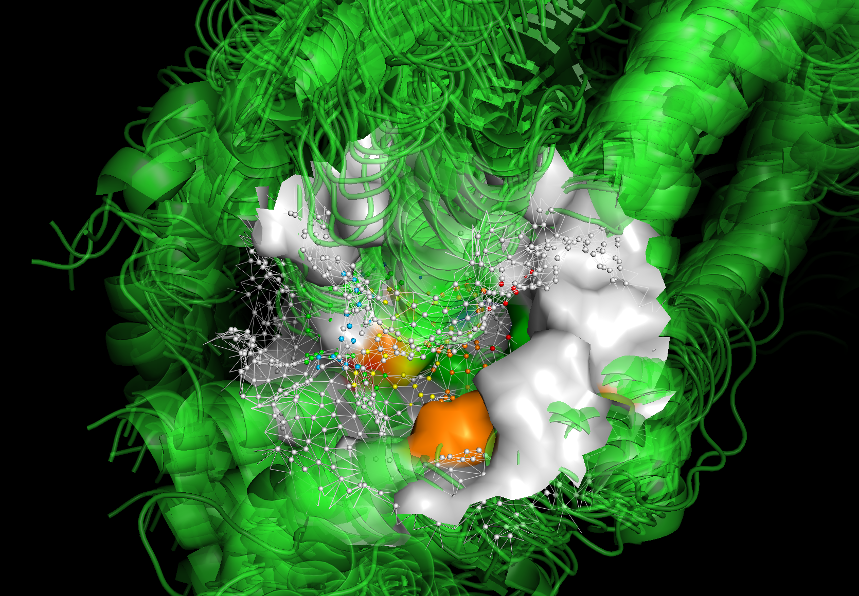
The visualization allows you to analyze the predictions across different frames of a protein ensemble. If it is an MD (Molecular Dynamics) trajectory, this visualization helps you understand how the structures—and specifically the fragment-binding regions—change over time.
In the example below, the visualization of the protein surface spans from the first frame to the last frame of the apo SMD trajectory, with an interval of 10 ns.
You may notice significant differences in the protein surfaces between:
The first frame, where the surface is colored by predicted fragment-binding regions.
The last frame, where the mesh and vertices are colored by predicted fragment-binding regions.
This comparison highlights how the protein surface and binding regions evolve throughout the trajectory.
Check the data (Apo_SMD_protein_vis_all.pse) by yourself in PyMOL if you are interested in the details.
# Here is a screenshot for the pymol visualization.
Image(filename=f"{project_root}/imgs/pymol_vis_02.png")
Conclusion#
Congratulations! You have now completed the tutorial. Here’s what you’ve achieved:
Loaded and Analyzed the Apo Trajectory
Used
TrajectoryHandlerandHoloDescriptorAnalyserto load and analyze the apo trajectory.
Used Parallel Processing for Efficiency
Leveraged parallel processing using
TrajHandlerPreprocessandTrajHandlerPredictionto process the full trajectory efficiently.
Identified Holo-like Conformations
Successfully identified holo-like conformations from an apo trajectory, which can serve as valuable protein ensembles for further drug design.
Next Steps#
This concludes all three tutorials. If you have any questions or encounter any issues, feel free to raise them on the GitHub repository.
Good luck with your research, and happy analyzing! 🚀